A System-Level Overview of Scale-up AI Infrastructure Racks (Part 1) — 中文解读

来源：Silicon Co-Design — A System-Level Overview of Scale-up AI Infrastructure Racks (Part 1: Network Architecture) 原文链接：https://www.siliconcodesign.com/p/a-system-level-overview-of-scale 原文发布日：2026-08-18 ｜ 作者：Silicon Co-Design 说明：本文为英文原文全文转载，附中文结构化解读。原文以英文写就，未作翻译；解读部分为整理归纳，不代表原作者观点。

第一部分：正文（Original Article）

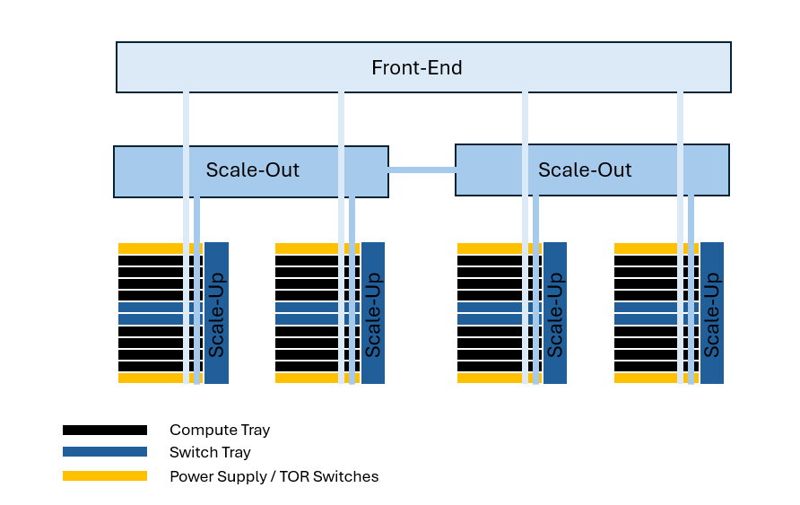图01｜原文配图（Silicon Co-Design）

This post is written to give system-context for the high-speed interconnect of AI rack architectures in preparation for Hot Interconnects and Hot Chips 2026 .

In part 1, I provide an overview of the network architecture:

• Front-End and Scale-Out - The Workhorses of Traditional Cloud Compute
• Why Scale-up - Massive BW for Tensor Parallelism
• Networking Terminology Physical Hardware Integration levels Switch Radix
• Tradeoffs in Fabric Complexity Co-Design Challenges Rack Architecture and Signal Integrity

Front-End and Scale-Out - The Workhorses of Traditional Cloud Compute

Why Scale-up - Massive BW for Tensor Parallelism

Networking Terminology

• Physical Hardware Integration levels
• Switch Radix

Physical Hardware Integration levels

Switch Radix

Tradeoffs in Fabric Complexity

• Co-Design Challenges
• Rack Architecture and Signal Integrity

Co-Design Challenges

Rack Architecture and Signal Integrity

I will cover compute parallelism and a few case studies in part 2.

This post is free and largely based on tutorials that can be found in their entirety at the Hot Chips 2025 website. Additionally, Hot Interconnects is this week which is free and online only. If you dial in, I encourage you to pass this around and use this as a reference guide to understand what is going on.

First, let me start with a quick note of my approach.

Bottom-Up is better for a more comprehensive understanding of the AI Rack

Unlike most people who cover rack systems from the top-down, I’ve taken a bottom-up approach where I’ve first written on the underlying subsystems from the chip level up to the board and system-levels. These include in-depth posts on high-speed optical / wireline communications , mixed signal IC , power , advanced packaging , AI accelerator fundamentals , and relevant business material to manage such complexity. Most of these underlying technologies are abstracted from outsiders because they are deep in the technical hierarchy and people within different specialty areas don’t always interact with other specialty areas.

However, as racks become more tightly integrated, designing components and subsystems within them requires a working knowledge of the entire rack architecture across abstraction levels. This includes understanding the historical context and cross-domain tradeoffs of adjacent technology areas to effectively co-design.

If you read my deep-dive posts, you will notice that I always talk about tradeoffs so that you not only know WHAT an architecture “is” (such as 800→48→12→1V for power), you understand WHY it arrived there and WHY it ISN’T something else. That is the essence of co-design engineering in my opinion that all engineers need to embrace. I also think understanding engineering tradeoffs as a non-engineer investor is important so that you can predict which way the wind will blow and allocate capital accordingly.

I’m always looking for writers with engineering background who cover such subsystems at depth to up-level how they play a role in the grand scheme of things. I find this challenging because it seems like most writing in AI infra that determine where capital flows is either macro-only or too technically in-depth.

Throughout this post, I link several of my deep dive posts throughout if you want to go more into depth into the topics I discuss. As always, if you’re an expert and notice a mistake, please reach out to me so I can fix it.

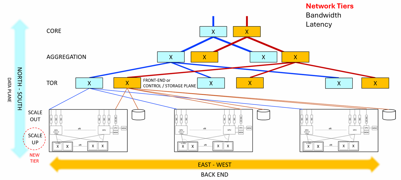图02｜原文配图（Silicon Co-Design）

Historically, most server racks utilized scale-out and front-end networks to handle data traffic between users and servers.

A front-end network connects all of the racks in the data center. It is responsible for managing north-south traffic that connects external clients, enterprise storage, and management systems to internal compute nodes.

Front-end networks handle north-south traffic using a 3-tier hierarchical network model , which is analogous to a postal system. This worked well when most web traffic was north-south (i.e. user-to-server), such as users requesting webpages from a server.

Front-end networks consist of the following three layers:

• Top-of-Rack (TOR) - The first entry point into the server for data Data goes through Tier 1 Switches which are directly attached to the GPUs
• Aggregation - The regional hub that multiple TOR switches connect to. These typically sit in separate network closets or central distribution racks Data is aggregated through Tier 2 Switches to connect multiple Tier 1 TOR switches when scaling out across racks or cluster pods
• Core - Moves massive volumes of data between major network blocks without causing bottlenecks. This is optimized for maximum data traffic throughput without running security protocols that can slow traffic down.

Top-of-Rack (TOR) - The first entry point into the server for data

• Data goes through Tier 1 Switches which are directly attached to the GPUs

Data goes through Tier 1 Switches which are directly attached to the GPUs

Aggregation - The regional hub that multiple TOR switches connect to. These typically sit in separate network closets or central distribution racks

• Data is aggregated through Tier 2 Switches to connect multiple Tier 1 TOR switches when scaling out across racks or cluster pods

Data is aggregated through Tier 2 Switches to connect multiple Tier 1 TOR switches when scaling out across racks or cluster pods

Core - Moves massive volumes of data between major network blocks without causing bottlenecks.

• This is optimized for maximum data traffic throughput without running security protocols that can slow traffic down.

This is optimized for maximum data traffic throughput without running security protocols that can slow traffic down.

Data is moved in the front-end network using either Ethernet or InfiniBand switches. A few examples of such switches used in AI include:

• InfiniBand - NVIDIA Quantum-X800 - Highest-performance, end-to-end 800 Gb/s networking designed for massive-scale AI
• Ethernet - Broadcom Tomahawk 5 - 51.2 TBps high-performance data center switch chip

InfiniBand - NVIDIA Quantum-X800 - Highest-performance, end-to-end 800 Gb/s networking designed for massive-scale AI

Ethernet - Broadcom Tomahawk 5 - 51.2 TBps high-performance data center switch chip

From Front-End to Scale-Out

Modern microservices such as Amazon and Netflix shifted the data movement to primarily east - west (server-to-server) that required high-bandwidth scale-out architectures.

Scale-out networking is essentially horizontal scaling—where data center capacity is expanded by interconnecting hundreds or thousands of independent compute nodes across a high-bandwidth, distributed switch fabric. This way, multiple compute nodes can work together on a single workload.

Scale-out primarily uses a flat leaf-spine topology that connects to GPU using network interface cards (NIC). These NICs convert GPU data into network packets and sends them to scale-out network switches.

Why Scale Up - Massive BW for Tensor Parallelism

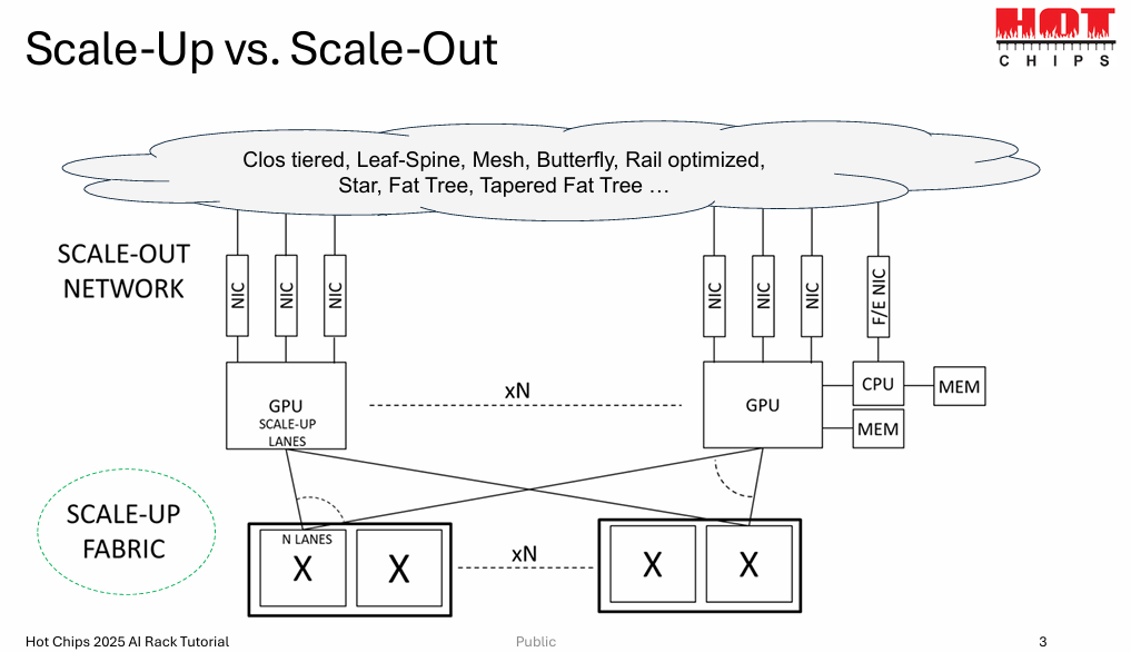图03｜原文配图（Silicon Co-Design）

AI compute greatly favors parallelism for computing massive amounts of MAC operations. Compute parallelism requires a lot of data movement during both training to distribute updated weights after each backpropagation pass and aggregate intermediate results. These will be discussed in more depth in part 2.

The problem with parallel computing in scale-out is that data movement is highly sensitive to latency with GPUs constantly “broadcasting” intermediate math results to each other. SW protocols in scale-out introduce unnecessary data routing micro-second latencies and packet drops to communicate between GPU A and B on the same cluster. This is bad for inference workloads that are latency sensitive.

Thus, scale-up emerged as a new high-bandwidth networking “tier” underneath the traditional 3-tier and scale-out hierarchy.

The scale-up domain has one job, and one job only:

To make multiple GPUs act like one massive virtual GPU with shared memory

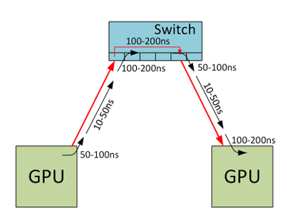图04｜原文配图（Silicon Co-Design）

Scale-up switches are low latency and operate on the order of ~100 nanoseconds compared to scale-out which operate at ~1 microsecond. Without a dedicated scale-up, all the data would choke the scale-out network and take forever to complete tasks.

There are many marketing terms used to describe scale-up fabric technologies. A few examples include:

• NVIDIA NVLink / NVLink Fusion
• Celestial AI Photonic Fabric
• Broadcom SUE - Scale-up Ethernet
• Ultra Accelerator Link (UALink)

NVIDIA NVLink / NVLink Fusion

Celestial AI Photonic Fabric

Broadcom SUE - Scale-up Ethernet

Ultra Accelerator Link (UALink)

Due to the massive amount of compute parallelism involved, most of the new market competitors and innovative technologies (such as optical and 448Gbps) optimize performance in the scale-up domain. Most high BW communication / computation want to be contained in the scale-up domain as much as possible. A new trend, Mixture of Experts, stresses scale-up even further due to sparse, unpredictable data patterns and the distributed nature of experts that also want to communicate in the scale-out domain.

Understanding and optimizing scale-up will make or break an AI cluster, and thus deserves special attention.

Networking Terminology

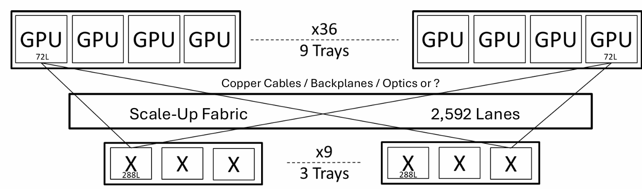图05｜原文配图（Silicon Co-Design）

Now I will define two important networking concepts.

Physical Hardware Integration Levels

In server rack systems, there is a standardized way to organize each component in server manufacturing integration levels using a L1 - L12 naming scheme. L1 - 5 refer to layers in the board and enclosure assembly, L6 - 9 refer to board and component populating, and L10 - 12 refer to system, rack, and cluster layers.

In the system context of AI racks, we care about the three highest levels:

• L10 (System/Tray Level): The single physical chassis or sled containing GPUs and local board switches
• L11 (Rack Level): The fully cabled rack frame housing multiple L10 trays
• L12 (Cluster / Multi-Rack Level): Connects multiple L11 racks together across the datacenter floor via scale-out optical networking (InfiniBand / RoCE switches)

L10 (System/Tray Level): The single physical chassis or sled containing GPUs and local board switches

L11 (Rack Level): The fully cabled rack frame housing multiple L10 trays

L12 (Cluster / Multi-Rack Level): Connects multiple L11 racks together across the datacenter floor via scale-out optical networking (InfiniBand / RoCE switches)

Switch Radix

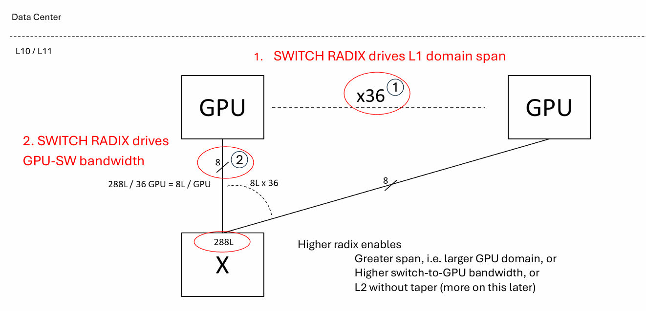图06｜原文配图（Silicon Co-Design）

In the switch tray, the switch radix refers to the total number of physical input and output ports (or high-speed links) integrated onto a single network switch chip. In modern GPU clusters, this radix is 288L total and uses a high-density SerDes switch architecture that connects 36 GPUs. Each connection typically has 8 lanes that most high-speed network interfaces and cabling commonly use.

The switch radix is critically important because it influences the amount of parallelism and therefore data BW that systems can handle. Switch radix introduces a number of constraints into the network architecture, including:

• L1 domain span - the total number of GPUs in parallel
• GPU-SW Bandwidth - the number of lanes each GPU can handle. 1.8 TB/s (224 GB/s aggregate throughput) is standard, but can increase if more lanes are added.

L1 domain span - the total number of GPUs in parallel

GPU-SW Bandwidth - the number of lanes each GPU can handle. 1.8 TB/s (224 GB/s aggregate throughput) is standard, but can increase if more lanes are added.

Examples of switch chips include:

• NVIDIA NVSwitch 4 ASIC - for traditional NVLink 5
• NVIDIA Quantum-X CPO Engine - for InfiniBand / Photonics
• Broadcom Tomahawk Ultra / Scale-Up Ethernet (SUE) ASICs
• Baya Systems NeuraScale Fabric Chips

NVIDIA NVSwitch 4 ASIC - for traditional NVLink 5

NVIDIA Quantum-X CPO Engine - for InfiniBand / Photonics

Broadcom Tomahawk Ultra / Scale-Up Ethernet (SUE) ASICs

Baya Systems NeuraScale Fabric Chips

Tradeoffs in Fabric Complexity

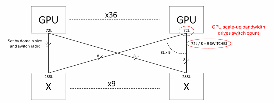图07｜原文配图（Silicon Co-Design）

There are several fundamental constraints that dictate the number of switches that can connect GPUs.

The switch radix governs the domain size and the number of GPUs that can be connected. Here we notice a span of 36 GPUs, each with 8 lanes, connecting to a 288L switch. Each GPU has up to 72 lanes to connect to 9 switches.

Multiple switches are used due to radix span and shoreline limitations of the SerDes. You cannot build a single mega-switch ASIC with 2,592 ports to connect to every GPU.

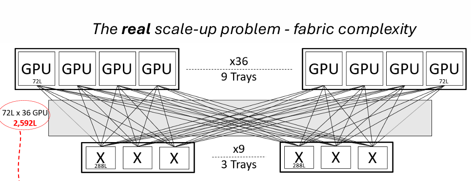图08｜原文配图（Silicon Co-Design）

There are several tradeoffs to scale performance with this configuration. Options include:

• Increasing the number of switches - this can increase BW, but add too many trays that cut into the number of compute trays
• Increasing the switch radix. This can support a larger number of GPUs, but this would require more SerDes, which is limited by shoreline limitations.

Increasing the number of switches - this can increase BW, but add too many trays that cut into the number of compute trays

Increasing the switch radix. This can support a larger number of GPUs, but this would require more SerDes, which is limited by shoreline limitations.

As a result, scale-up clusters limit the # of switches and accept that there will be a BW limitation on how many GPUs talk to each other simultaneously.

In addition, there are also several co-design challenges in scale-up clusters due to cross-domain interactions, including:

• Mechanical - Weight of rack, manufacturability, yield, how many lanes can physically exit switch and compute sleds
• Thermal / Cooling - More power hungry GPUs in a tighter area need heat removed out of the rack, and liquid cooling requires failsafe mechanisms
• Power - size of bus bar, safety
• Signal Integrity - affected by mechanical form factor and cable length. Long signal paths need retimers that add additional power, mechanical, and thermal considerations

Mechanical - Weight of rack, manufacturability, yield, how many lanes can physically exit switch and compute sleds

Thermal / Cooling - More power hungry GPUs in a tighter area need heat removed out of the rack, and liquid cooling requires failsafe mechanisms

Power - size of bus bar, safety

Signal Integrity - affected by mechanical form factor and cable length. Long signal paths need retimers that add additional power, mechanical, and thermal considerations

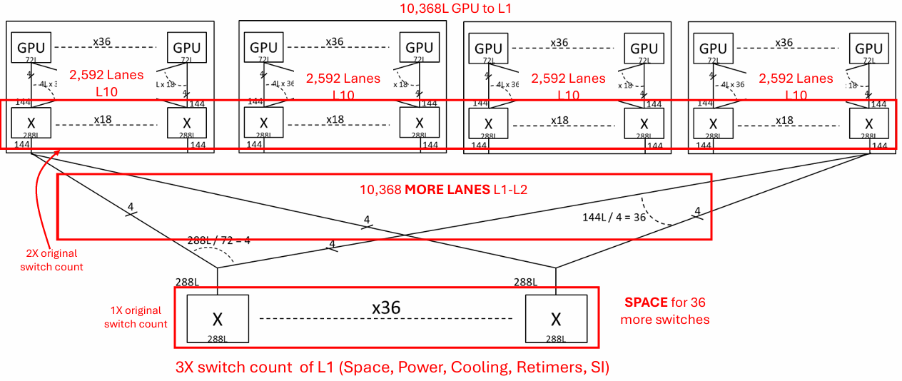图09｜原文配图（Silicon Co-Design）

To further increase parallelism, there are several approaches to scale-up multiple “domains” with L1 and L2 switches. Since each scale-up switch has 288L, parallelizing four scale-up domains blows up the required switch complexity needed to handle every single possible GPU-GPU combination. There are several alternative topologies to this such as L1.5 with more information in the slide deck.

Rack Architecture and Signal Integrity

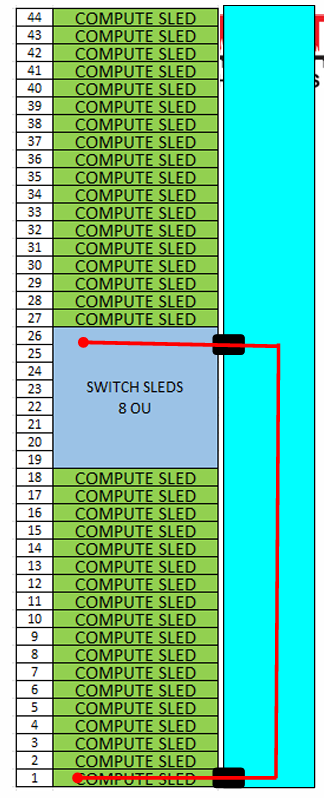图10｜原文配图（Silicon Co-Design）

All of these switches have to fit into the rack to accommodate both switch and compute.

In a standard GB200/300 rack, there are 44 slots. Aside from required rack peripherals, each rack slot can comprise of either a compute sled or a switch sled. Each compute sled consists of 2-4 GPUs and 1-2 CPUs and associated peripherals (power, high speed comm, heatsinks, and management circuitry) for either 1OU or 2OU height configurations.

In legacy web-server racks, switches sat at the Top-of-Rack (ToR). To minimize copper reach in AI datacenter racks, rows 19 - 26 are reserved for the switches and the rest above and below it for compute and power / peripheral trays. This improves signal integrity as data rates increase as copper faces several challenges for longer reaches.

As many people note, copper is reaching a physical speed and length limit, which makes optical such an attractive option for high-speed and low latency interconnect.

When designing the scale-up network, the rule of thumb is “use copper where you can, and optics where you must”. Pluggable optical transceivers (OSFP / QSFP-DD) for scale-up are expensive and power hungry and are generally minimized, despite investors appetite for more of them.

With increasing data rates, it’s becoming increasingly challenging to use copper within the PCB itself, and thus co-packaged optics is emerging as a potential scaling solution. Here are in-depth posts that cover two major classes of modulators being considered for CPO:

Conclusion

Scale-up is critically important in AI compute performance. Everything - from data BW, latency, mechanical, thermals - are all factors in AI performance.

In Part 2, I will discuss four different forms of parallelism, including Mixture-of-Experts, as well as several rack and model case examples. Stay tuned for that.

第二部分：解析（深度解读）

以下为基于原文的结构化中文解读，仅供学习交流，不代表原作者观点。

一、这篇文章在讲什么

作者（Silicon Co-Design）赶在 Hot Interconnects / Hot Chips 2026 之前，给 AI 机架的高速互连做了一层「系统级背景铺垫」。本文是 Part 1，只讲网络架构，刻意不碰计算并行与具体案例（留到 Part 2）。核心信息很明确：Scale-up（纵向扩展——把一颗「逻辑大模型」铺在多颗加速芯片上协同算）对互连带宽的需求，正在反过来重塑整个机架的网络拓扑、交换机 radix、物理集成方式与信号完整性设计。

二、关键概念拆解

• Front-End / Scale-Out 与 Scale-Up 的分工：传统云算力靠前端网络（Front-End，连接用户与存储）和 Scale-Out（横向扩展，节点间通信）干活；但大模型训练/推理里「单任务内部的通信」走的是 Scale-Up——把张量并行、专家并行等切开的算子，在极近距离内以极高带宽互通。两者带宽量级与延迟预算完全不同。
• 为什么 Scale-up 要巨大带宽：张量并行（Tensor Parallelism）每一步前向/反向都要在切分维度上做 All-Reduce / All-Gather，通信量正比于激活值大小，频率正比于计算步速。模型越大、步越快，Scale-up 域的聚合带宽需求就呈指数级膨胀。
• 网络术语与物理集成层级：从 die → 封装内（In-package）→ 板级（PCB）→ 背板/前面板 → 机架（Rack）多层集成，每一层的信道损耗、走线密度、可制造性都不一样。
• 交换机 Radix 的硬限制：单颗交换芯片的端口数（radix）有限，决定了一个 Scale-up 域能挂多少颗加速芯片；radix 不够就得叠多层交换，代价是跳数、延迟与功耗。
• 织物复杂度 vs 协同设计：全互连（full mesh）最简单但 radix 爆炸；树形/胖树省 radix 却引入阻塞与不对称的拥塞。作者强调这是「协同设计」问题——网络拓扑、路由、流控必须和并行策略、集合通信库一起定。
• 机架架构与信号完整性：当单通道带宽推到几百 Gb/s、走线以米计，Insertion Loss、串扰、反射、抖动成为硬约束——这也正是先进封装（CoWoS 类）、共封装光学（CPO）、更激进背板方案被反复讨论的物理根源。

三、与本站其他文章的衔接

• 光互联 / CPO 系列：Scale-up 域的带宽密度，正是 CPO、硅光收发器、DWDM 微环（见本批另一篇 Intel VLSI 2026 MRR-DWDM）登场的根本驱动力——电互连在「带宽 × 距离 × 功耗」三角上已经吃紧。
• SerDes 系列：信号完整性那一节，落到物理层就是更高速 SerDes（224/448 Gbps）与均衡技术。
• 先进封装系列：物理集成层级里「封装内互连」一节，直接对应 CoWoS-L、EMIB 等 2.5D/3D 方案。

四、趋势与投资映射

• 投资主线不是「哪颗交换芯片赢」，而是 Scale-up 域的带宽墙 会持续把价值推向：先进封装、硅光/CPO、高速 SerDes，以及能降低织物复杂度的拓扑/路由 IP。
• 风险：radix 与功耗的军备竞赛，可能让「全互连」方案在大规模下不可持续；任何声称「纯 CPO 股」的判断，都应回到这篇系统级视角来审视。