MicroZed Chronicles: Looking Beyond the FFT — 越过 FFT 之后：用瀑布图给频谱加上时间维度

本文翻译并转载自 Adiuvo Engineering（作者 Adam Taylor）的博客文章 MicroZed Chronicles: Looking Beyond the FFT，原文发布于 2026-07-29。 结构为 英文原文 + 中文翻译，供中英对照学习。原文链接：https://www.adiuvoengineering.com/post/microzed-chronicles-looking-beyond-the-fft 文末站方的课程 / 开发板 / 书籍等导航链接已略去，仅保留文章主体与 FPGA Horizons 大会信息。著作权归原作者所有，翻译仅供学习参考。

---

第一部分：正文（Original Article）

MicroZed Chronicles: Looking Beyond the FFT

FPGA Horizons London — October 6th and 7th 2026 — get Tickets here.

The $99 Artix UltraScale+ Explorer Board — learn more here

Over the last few blogs we have been looking at element of DSP and signal processing, especially elements which allow us to work in the frequency domain such as Filters and Fourier Transforms.

I have also been experimenting a little recently with the Opal Kelly XEM7320, and FrontPanel which is very interesting for visualisation.

So using the XEM7320 fitted with a SYZYGY SZG-ADC pod containing a LTC2264-12 dual channel ADC. I thought it would be good to create an example which allows us to understand how we can extract more information from the frequency domain.

To do this I created the ADC interface in RTL, connected it through an FFT to the FrontPanel IP core, and developed a FrontPanel application on the host to pull out the results of the FFT.

In this blog I want to step back a little from implementation detail and focus on what we do with those FFT frames once we have them, because how we present spectral data matters just as much as how we capture it.

I will make the Vivado design, IP cores, and FrontPanel App available on my GitHub if you a want to examine them in more detail.

The Limitation of a Single Spectrum

As we have seen the FFT is one of the key elements of FPGA signal processing. To use it we give it a block of samples and the result tells us the amplitude present at each frequency across the first Nyquist zone. In the example I created we are sampling at 40 MS/s with a 4096 point FFT in the fabric, which gives me a bin resolution of 9.766 kHz across DC to 20 MHz.

The problem is that a single FFT frame is a snapshot taken at one point in time, it does not contain any history.

The FFT output tells us what the spectrum looked like during one 102.4 microsecond window and nothing more. If the signal environment is stationary, a sine wave sitting at a fixed frequency for example, a snapshot is perfectly adequate, and indeed it is exactly what we use for ADC dynamic testing where we compute SNR, SFDR and ENOB from a coherent capture.

Real signal environments are rarely that accommodating however, signals sweep, hop, pulse on and off, and change amplitude. Interference arrives, misbehaves for a few milliseconds and disappears again. A spur may be present in one capture and absent in the next, and with a single spectrum we have no way of knowing whether if we saw a persistent problem or a one-off event. Anyone who has chased an intermittent EMC issue with a spectrum analyser in single sweep mode will know this frustration.

We can see the history of the FFT frame by using a waterfall display this by adding the missing dimension, time. Each FFT frame becomes one row of an image, frequency runs along the horizontal axis, capture order runs down the vertical axis, and amplitude in dBFS is mapped to colour. The spectrum stops being a photograph and becomes a film, and entire classes of behaviour that are invisible in a snapshot become more visible.

The System Behind the Display

Before looking at the waterfall diagram let me first explain the design in the XEM7320 FPGA. The RTL interface to the ADC handles the LTC2264-12 in its default two lane, 16 bit serialisation mode. The pod returns a 160 MHz DCO alongside the serial data, giving a bit rate of 320 Mbit/s per lane, in the Artix-7 I use the SelectIO 8:1 DDR to perform the deserialisation.

The ADC IP core then detects the frame pattern rotation, aligns all lanes to the same sample boundary, reconstructs the 12 bit samples and presents both channels as a 32 bit AXI4-Stream master through a small asynchronous FIFO.

As the ADC needs to be configured at start up / reset an SPI sequence configures and verifies the ADC. This means the interface comes up ready to stream without host involvement, simplifying integration. The configuration of the ADC over the SPI can be achieved by using generics in VHDL.

The ADC IP Core out stream is input into a 4096 point FFT, and the complex results are made available to the host through the FrontPanel IP core over a block pipe. Here we needed to create a simple AXIS to Block Pipe necessary for the FP IP Core in the FPGA.

At first I created a simple FPApp which shows the waterfall diagram as it was captured. This is useful but I wanted to be able to demonstrate why waterfall diagrams are useful. Hence I need to be able to control both the XEM7320 capture and the signal generation.

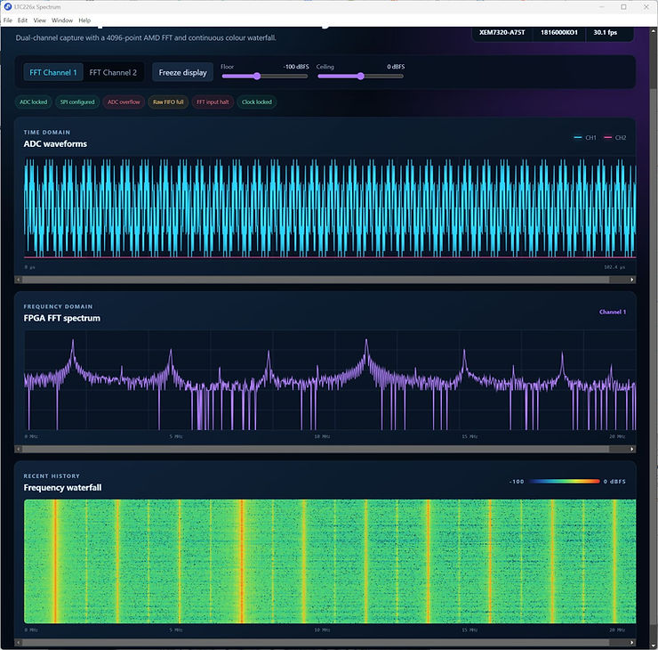
To ensure I could do this I created a python script which allows me to control both the XEM7320 and the waveform generator.

Using the same Python script ensures both stimulus and capture are coordinated as a single script performs both function.

What the Waterfall Reveals

To demonstrate why the time axis earns its keep, the python application runs three scripted scenarios, each producing a 72 row waterfall.

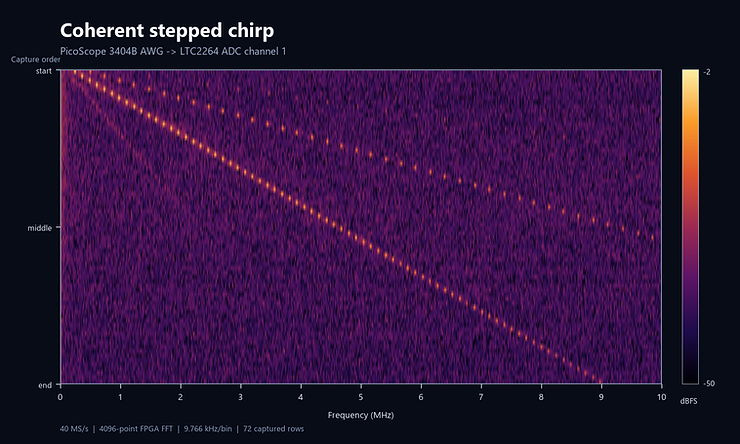
The first is a coherent stepped chirp from 0.25 MHz to 9 MHz. On the waterfall this appears as a clean diagonal line marching across the band, and the constant slope immediately confirms that the step sequencing and the row capture are behaving. More interesting is the second, fainter diagonal running at twice the slope. That is the second harmonic of the generated tone, and the waterfall identifies it without any analysis at all, because a harmonic must track the fundamental at an integer multiple of its trajectory. This is a genuinely powerful diagnostic technique. Different spur mechanisms trace different paths as the input moves. Harmonics run at multiples of the fundamental slope, while images and interleaving artefacts reflect about Nyquist and run with the opposite slope. A single spectrum shows you a spur; a waterfall under a swept stimulus tells you what kind of spur it is.

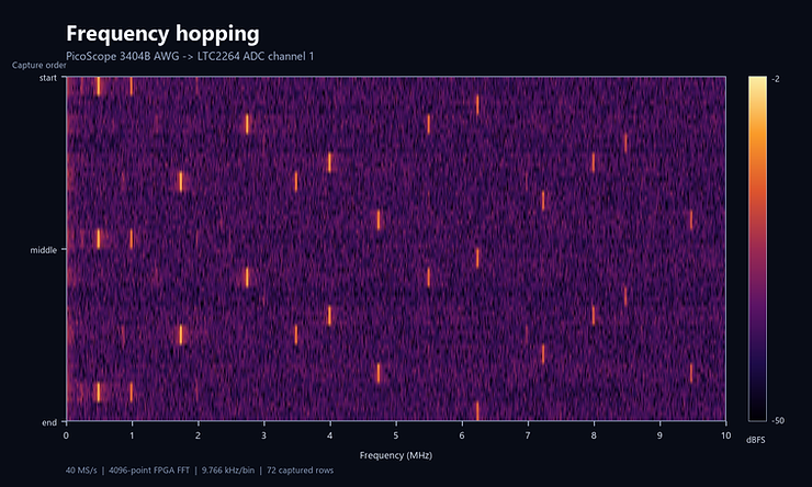
The second scenario is a deterministic frequency hopping sequence. Here the waterfall shows short dashes scattered across the frequency axis, each one a dwell at a pseudo random frequency. Try to characterise this signal with individual spectra and you would see a single unexplained tone in each capture, at a different frequency every time, which looks indistinguishable from intermittent interference. The waterfall makes the structure unmistakable, revealing the dwell time, the hop set and the repetition of the pattern. Frequency agility is a staple of modern communications and of the radar world I spent many years in, and the waterfall is the natural way to observe it.

The third scenario combines tone bursts separated by silence with a sequence of amplitude coded hops. The bursts appear as short vertical strokes with genuinely quiet rows between them, which also serves as a useful check on the noise floor of the capture chain when no stimulus is present. The amplitude coded section then shows the same colour scale doing double duty, with the brightness of each dwell reflecting the programmed level. Time gated behaviour of this kind, signals that switch on and off, is completely opaque to a snapshot, because the answer to what the spectrum contains genuinely depends on when you ask.

Wrapping Up

None of the three examples above can be easily described by a single FFT frame, and between them they cover a large fraction of the signals we actually encounter, whether we are verifying an ADC front end, hunting an intermittent spur, or observing a frequency agile emitter.

The waterfall costs us very little. The fabric was already producing FFT frames faster than we could use them, and the host simply has to keep the rows honest and paint them. In return it converts the FFT from an instrument that answers what is present into one that answers what is happening, and that is usually the question we actually wanted answered.

With the XEM7320 and the SYZYGY ADC pod, the whole chain from LVDS deserialisation to a live waterfall runs on a compact, low cost platform, and the FrontPanel integration means the host side is a few hundred lines of Python rather than a driver development exercise. In future blogs we will build on this foundation, as there is plenty more we can do once the spectrum has a time axis.

FPGA Horizons London — October 6th and 7th 2026 — get Tickets here.

---

第二部分：翻译（中文）

MicroZed Chronicles：越过 FFT 之后

FPGA Horizons London —— 2026 年 10 月 6–7 日 —— 购票 见此。

99 美元的 Artix UltraScale+ Explorer 开发板 —— 了解更多 见此。

在最近的几篇博客里，我们一直在看 DSP 与信号处理的要素，尤其是那些让我们能在频域工作的模块，比如滤波器与傅里叶变换。

最近我也用 Opal Kelly XEM7320 和 FrontPanel 做了点实验，后者在可视化方面非常有趣。

于是我用装有 SYZYGY SZG-ADC pod（内含 LTC2264-12 双通道 ADC）的 XEM7320，做了一个示例，帮助理解我们如何能从频域提取更多信息。

为此，我在 RTL 里写了 ADC 接口，把它经 FFT 连到 FrontPanel IP 核，并在主机上开发了 FrontPanel 应用来取出 FFT 的结果。

在这篇博客里，我想稍微退一步，不谈实现细节，而是聚焦在拿到 FFT 帧之后我们该拿它们做什么——因为如何呈现频谱数据，和我们如何捕获它同样重要。

如果你想要更深入研究，我会把 Vivado 设计、IP 核和 FrontPanel 应用放到我的 GitHub 上。

单一频谱的局限

正如我们所见，FFT 是 FPGA 信号处理的关键模块之一。使用它时，我们喂给它一块采样，结果告诉我们第一奈奎斯特区内每个频率上的幅度。在我做的例子里，我们以 40 MS/s 采样、在 FPGA 内做 4096 点 FFT，得到 DC 到 20 MHz 上 9.766 kHz 的 bin 分辨率。

问题在于，单帧 FFT 是在某个时刻拍下的一张快照，它不含任何历史。

FFT 输出只告诉我们，在一段 102.4 微秒的窗口里频谱是什么样子，仅此而已。如果信号环境是平稳的——比如一个固定频率上的正弦波——一张快照就完全够用，事实上这正是我们在 ADC 动态测试中所用的：从相干捕获里计算 SNR、SFDR 和 ENOB。

然而真实的信号环境很少这么配合：信号会扫频、跳频、脉冲式开关，幅度也会变化。干扰来了，捣乱几毫秒又消失。一个杂散（spur）可能在这帧里有、下一帧没有；而单帧频谱我们无法判断自己看到的是持续性问题还是偶发事件。任何用频谱仪单扫模式追过间歇性 EMC 问题的人，都懂这种挫败。

我们可以通过瀑布图（waterfall display）看到 FFT 帧的历史——补上缺失的那一维：时间。每一帧 FFT 成为图像的一行，频率沿水平轴展开，捕获顺序沿垂直轴向下，幅度（dBFS）映射成颜色。频谱不再是一张照片，而变成了一部电影，一整类在快照里看不见的行为变得可见。

显示背后的系统

在看瀑布图之前，先解释一下 XEM7320 FPGA 里的设计。到 ADC 的 RTL 接口以默认的两条 lane、16 位串行化模式处理 LTC2264-12。pod 返回 160 MHz 的 DCO 以及串行数据，每 lane 比特率 320 Mbit/s；在 Artix-7 上我用 SelectIO 8:1 DDR 做解串行。

ADC IP 核随后检测帧模式旋转，把所有 lane 对齐到同一采样边界，重建出 12 位采样，并通过一个小异步 FIFO 把两路通道以 32 位 AXI4-Stream master 的形式送出。

由于 ADC 需要在启动 / 复位时配置，一段 SPI 序列会配置并校验 ADC。这意味着接口上电即可流送，无需主机介入，简化了集成。ADC 的 SPI 配置可以通过 VHDL 中的泛型（generics）实现。

ADC IP 核的输出流进入一个 4096 点 FFT，复数结果通过 FrontPanel IP 核经 block pipe 提供给主机。这里我们需要为 FPGA 里的 FP IP 核做一个简单的 AXIS-to-Block-Pipe 转换。

起初我做了一个简单的 FPApp，实时显示捕获到的瀑布图。这有用，但我想演示瀑布图为何有用，因此我需要能同时控制 XEM7320 的捕获和信号生成。

为此我写了一个 Python 脚本，让我能同时控制 XEM7320 和波形发生器。

用同一个 Python 脚本确保激励与捕获协调一致，因为单个脚本同时完成这两个功能。

瀑布图揭示了什么

为了演示时间轴为何物有所值，该 Python 应用运行三个脚本化场景，每个生成 72 行的瀑布图。

第一个是 0.25 MHz 到 9 MHz 的相干步进线性调频（chirp）。在瀑布图上它表现为一条斜穿频带的干净对角线，恒定的斜率立刻确认了步进序列与行捕获都在正常工作。更有意思的是第二条更淡的、以两倍斜率运行的对角线——那是所产生音调的二次谐波，瀑布图无需任何分析就识别了它，因为谐波必须以其轨迹的整数倍跟踪基波。这是一种真正强大的诊断技术。当输入移动时，不同的杂散机制走出不同的路径：谐波以基波斜率的整数倍运行，而镜像与交织伪像则关于奈奎斯特频率反射、以相反斜率运行。单帧频谱只给你一个杂散；扫频激励下的瀑布图告诉你它是什么类型的杂散。

第二个场景是一个确定性的跳频序列。这里瀑布图显示沿频率轴散布的短横线，每一条都是在一个伪随机频率上的驻留（dwell）。若用单帧频谱去刻画这个信号，你会在每次捕获里看到一个孤立的、频率不断变化的音调，和间歇性干扰难以区分。瀑布图让结构一目了然，揭示出驻留时间、跳频集合与模式的重复。频率捷变是现代通信以及我待过多年的雷达领域的家常便饭，而瀑布图正是观察它的天然方式。

第三个场景把被静默隔开的音调突发（tone bursts）与一段幅度编码的跳频序列结合起来。突发表现为短竖线，其间是真正安静的行——当没有激励时，这也顺便检验了捕获链的本底噪声。幅度编码部分则让同一套颜色刻度身兼两职，每个驻留的亮度反映其编程设定的电平。这种时间门控行为——开关的信号——对快照完全不透明，因为”频谱里有什么”的答案真的取决于你何时问。

总结

上面三个例子没有哪一个能被单帧 FFT 轻易描述，而它们合起来覆盖了我们实际上遇到的信号的很大部分——无论我们是在验证 ADC 前端、追查间歇性杂散，还是观察一个频率捷变的发射机。

瀑布图的成本极低。FPGA fabric 产生 FFT 帧的速度本就超过我们能消费的速度，主机只需诚实地维护各行并把它们画出来。作为回报，它把 FFT 从”回答有什么存在”的仪器，变成了”回答正在发生什么”的仪器——而那通常才是我们真正想问的问题。

借助 XEM7320 和 SYZYGY ADC pod，从 LVDS 解串行到实时瀑布图的整条链路都跑在一个紧凑、低成本的平台上；FrontPanel 的集成意味着主机侧只是几百行 Python，而非一场驱动开发。在未来的博客里我们会在此基础上继续，因为一旦频谱有了时间轴，我们还能做很多事。

FPGA Horizons London —— 2026 年 10 月 6–7 日 —— 购票 见此。