Applying Mixture of Experts in LLM Architectures — 在 LLM 中应用混合专家(MoE)
NVIDIA 技术博客详解 MoE(混合专家)架构:如何用多个专家子网络在扩大模型容量的同时降低每 token 计算成本,并以开源 Mixtral 8x7B 实证专家的专业化行为。附英文原文、本地化图表与中文深度解读。
原文:Applying Mixture of Experts in LLM Architectures,作者 Kyle Kranen 与 Vinh Nguyen(NVIDIA Technical Blog),发布于 2024-03-14。 本页结构:第一部分为英文原文(Original Article,含 NVIDIA 官方图表,已本地化),第二部分为中文深度解读(解析)。 说明:原文无付费墙,全文完整收录;图片来自 developer-blogs.nvidia.com,已下载至本站 assets。
第一部分:正文(Original Article)
Mixture of experts in LLM architectures
This section provides some background information and highlights the benefits of using MoE in LLM architectures.
Model capacity
Model capacity can be defined as the level of complexity that a model is capable of understanding or expressing. Generally, models with larger numbers of parameters (when sufficiently trained) have historically proven to have larger capacity.
How does MoE factor into capacity? Models with more parameters generally have greater capacity, and MoE models can effectively increase capacity relative to a base model by replacing layers of the model with MoE layers in which the expert subnetworks are the same size as the original layer.
Researchers have investigated the accuracy of MoE models against fully dense models of similar size trained on the same amount of tokens (MoE size: E*P parameters compared to fully dense size: EP parameters). The fully dense models generally outperform, although this is still an active area of research. For more details, see Unified Scaling Laws for Routed Language Models.
This raises the question, why not just use a dense model? The answer here lies in sparse MoE, and specifically the fact that sparse MoEs are more flop-efficient per parameter used.
Consider Mixtral 8x7B, a model that uses eight-expert MoE, where only two experts are used for each token. In this case, in any given forward pass of a single token within the model, the number of parameters used for any given token in a batch is much lower (12 billion parameters used of a total 46 billion parameters). This requires less compute compared to using all eight experts or a similarly-sized fully dense model. Given that tokens are batched together in training, most if not all experts are used. This means that in this regime, a sparse MoE uses less compute and the same amount of memory capacity compared to a dense model of the same size.
In a world in which GPU hours are a highly coveted resource, training a fully dense model over a massive scale is prohibitively expensive in terms of both time and cost. The Llama 2 set of models (fully dense) trained by Meta reportedly spent 3.3 million NVIDIA A100 GPU hours in pretraining. To put this in context, 3.3 million GPU hours on 1,024 GPUs at full capacity with no downtime would take approximately 134 days. This does not account for any experimentation, hyperparameter sweeps, or training interruptions.
MoE trains larger models while reducing cost
MoE models help reduce cost by being more flop-efficient per weight, meaning that under regimes with fixed time or compute cost constraints, more tokens can be processed and the model can be further trained. Given that models with more parameters need more samples to fully converge, this essentially means that we can train better MoE models than dense models on a fixed budget.
MoE provides decreased latency
With large prompts and batches where computation is the bottleneck, MoE architecture can be used to deliver decreased first-token serving latency. Latency decreases are made even more important as use cases like retrieval-augmented generation (RAG) and autonomous agents may require many calls to the model, compounding single-call latency.
How do MoE architectures work?
Two key components contribute to MoE models. First, the “expert” subnetworks that compose the mixture, which are used for both dense and sparse MoE. Second, the routing algorithm used by sparse models to determine which experts process which tokens. In some formulations for dense and sparse MoE, the MoE may include a weighting mechanism that is used to perform a weighted average of expert outputs. For the purpose of this post, we will focus on the sparse case.
In many published papers, the MoE technique is applied to Multi-Layer Perceptrons (MLPs) within transformer blocks. In this case, the MLP within the transformer block is usually replaced with a set of expert MLP subnetworks, the results of which are combined to produce the MLP MoE output using averaging or summation.
Research has also suggested that the concept of MoE can be extrapolated to other parts of the transformer architecture. The recent paper SwitchHead: Accelerating Transformers with Mixture-of-Experts Attention suggests that MoE can also be applied to the projection layers that transform inputs into Q, K, and V matrices to be consumed by the attention operation. Other papers have proposed the application of the conditional execution MoE concept to the attention heads themselves.
Routing networks (or algorithms) are used to determine which of the experts are activated in the case of a particular input. Routing algorithms can vary from simple (uniform selection or binning across average values of tensors) to complex, as explained in Mixture-of-Experts with Expert Choice Routing.
Among many factors that determine the applicability of a given routing algorithm to a problem, two core factors are often discussed: model accuracy under a specific routing regime and load balancing under a specific regime. Choosing the right routing algorithm can be a trade-off between accuracy and flop efficiency. A perfectly load-balanced routing algorithm might reduce the accuracy per token, while the most accurate routing algorithm might unevenly distribute tokens between experts.
Many proposed routing algorithms are designed to maximize model accuracy while minimizing the bottleneck presented by any given expert. While Mixtral 8x7B uses a Top-K algorithm to route tokens, papers such as Mixture-of-Experts with Expert Choice Routing introduce concepts to ensure that experts are not overly routed to. This prevents the formation of bottlenecks.
Experimenting with the Mixtral model
In practice, what does each expert learn? Do they specialize in low-level lingual constructs, such as punctuation, verbs, adjectives, and so forth, or are they the masters of high-level concepts and domains, such as coding, math, biology, and law?
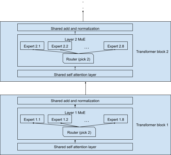
To this end, we designed an experiment using the Mixtral 8x7B model. This model has 32 sequential transformer blocks, wherein each MLP layer is replaced with a sparse MoE block with eight experts, of which only two are activated for each token. The remaining layers, including self-attention and normalization layers, are shared by all the tokens.
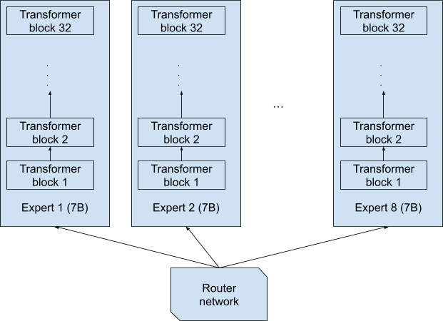
It is worth noting that when reading the name 8x7B, one could imagine the experts being eight separate full networks, each of 7 billion parameters, and each token is fully processed end-to-end by one of these eight full networks (Figure 1). This design would yield an 8x7B = 56B model.
1
	**Figure 1. A possible interpretation of the Mixtral 8x7B model**
While this is certainly a plausible design, it wasn’t the one used in Mixtral 8x7B. The actual design is depicted in Figure 2, with each token processed by 7 billion parameters. Note that a token and its copy (which is processed by the second-picked expert at each layer) is processed by only 12.9 billion parameters in total, not 2x7B = 14B. And the whole network is only 47 billion, not 8x7B = 56B parameters, due to the shared layers.
1
	**Figure 2. Simplified Mixtral 8x7B model architecture**
Therefore, each of the tokens passing through the network must go through a lattice-like structure, with (\binom{8}{2} = 28) possible combinations of two experts at each layer. Mixtral 8x7B has 32 transformer blocks, thus there are a total of (28^{32}) possible instantiations of the network.
If we consider each of these instantiations as a “full-stack expert” (one that processes a token end to end), is it possible to find out what expertise they offer? Unfortunately, since 28^{32} is a really large number (~2×10^{46}), which is orders upon orders of magnitude larger than all the data used to train LLMs (~3T to 10T tokens for most LLMs), rarely will any two tokens be processed by the same instantiation. Thus, we will study what each layer expert specializes on as opposed to each full expert combination.
Experimental results
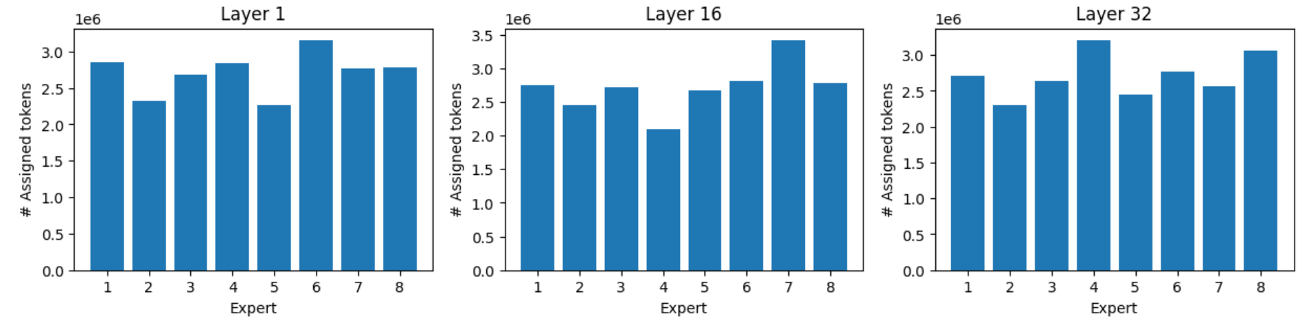
We ran all the samples of the Massive Multitask Language Understanding (MMLU) benchmark through the model. This includes multiple-choice questions on 57 topics, as diverse as abstract algebra, world religions, professional law, anatomy, astronomy, and business ethics, to name a few. We recorded the token-expert assignment for each of the eight experts on layers 1, 16, and 32.
Upon parsing the data, several observations are worth noting.
Load balancing
Thanks to load balancing, the experts receive equalized loads, yet the most busy expert still receives up to 40–60% more tokens than the least busy one.
1
	**Figure 3. Expert loading distribution over all MMLU topics**
Domain-expert assignment
Some domains activate some experts more than others.
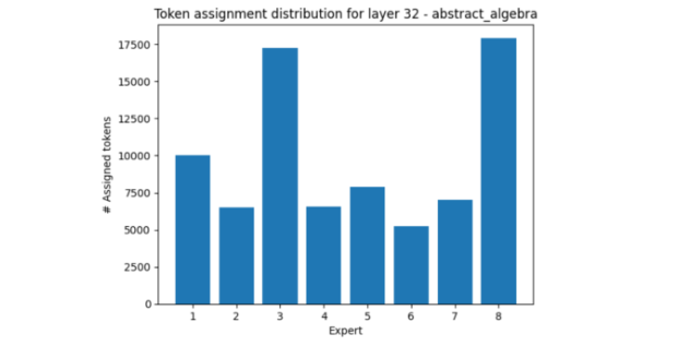
In layer 32, one such example is abstract algebra, which makes use of experts three and eight much more than others.
1
	**Figure 4. Token distribution over expert in layer 32 for abstract algebra**
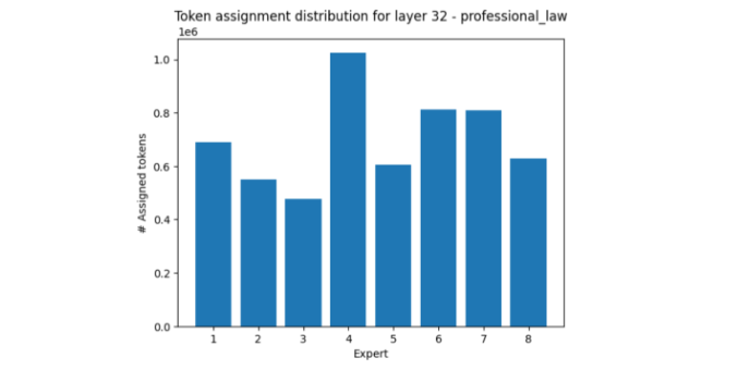
The area of professional law, on the other hand, mostly activates expert four while muting experts three and eight, relatively.
1
	**Figure 5. Token distribution over expert in layer 32 for professional law**
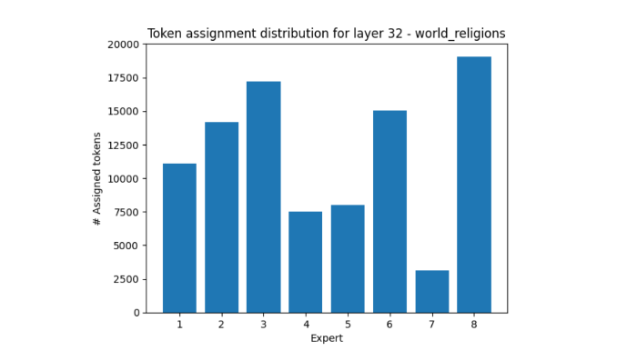
World religions is another fascinating example, in that expert seven receives more than 5x less tokens than expert eight.
1
	**Figure 6. Token distribution over expert in layer 32 for world religions**
These experimental results show that the experts’ load distribution tends towards uniformity across a diverse range of topics. However, when samples all fall exclusively under a certain topic, there could be a large distributional imbalance.
Most preferred tokens by experts
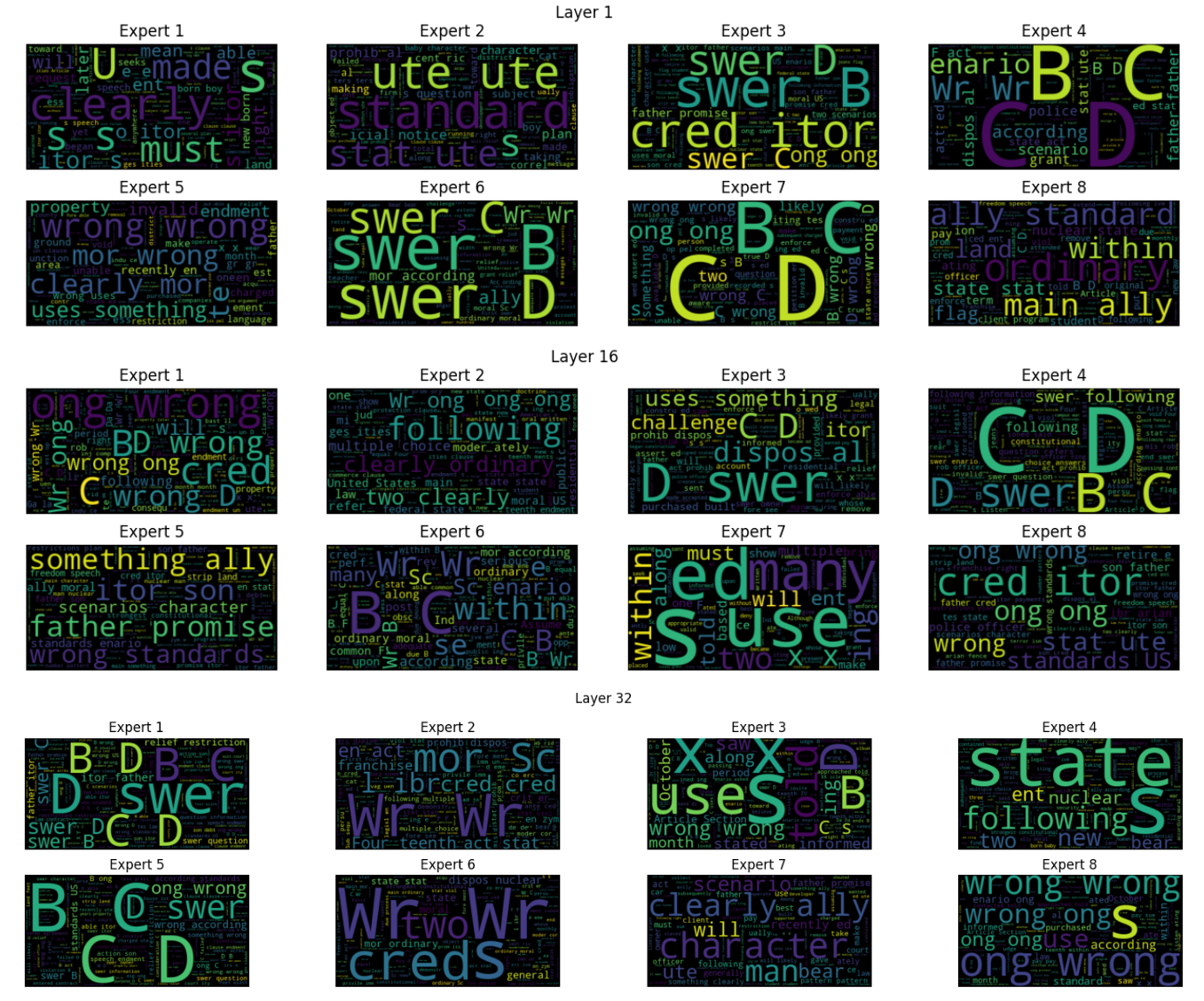
The word cloud in Figure 7 shows which tokens were most frequently processed by each expert.
1
	**Figure 7. Most common tokens processed by experts**
Most preferred experts by tokens
Does each token have a preferred expert? Each token seems to have a more preferred set of experts, as the following examples show.
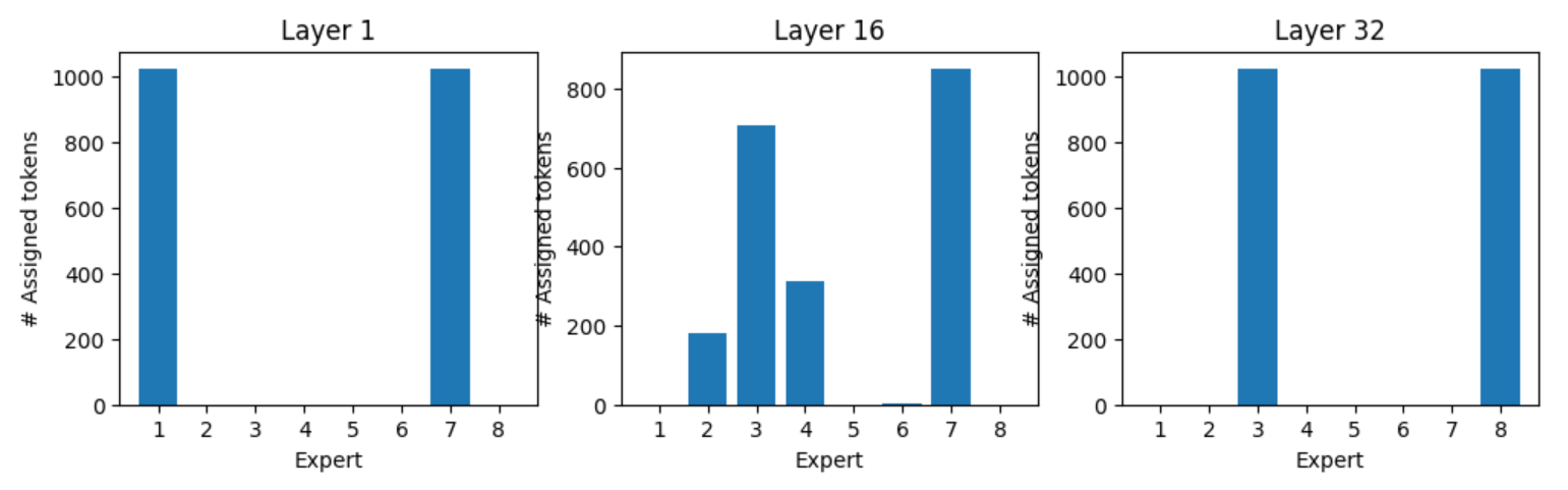
Expert assignment for token “:” , all “:” tokens are processed by experts one and seven in layer one, and experts three and eight in layer 32 (Figure 8). Figures 9, 10, and 11 show the expert assignment for various tokens.
1
	**Figure 8. Expert assignment for token “:”**
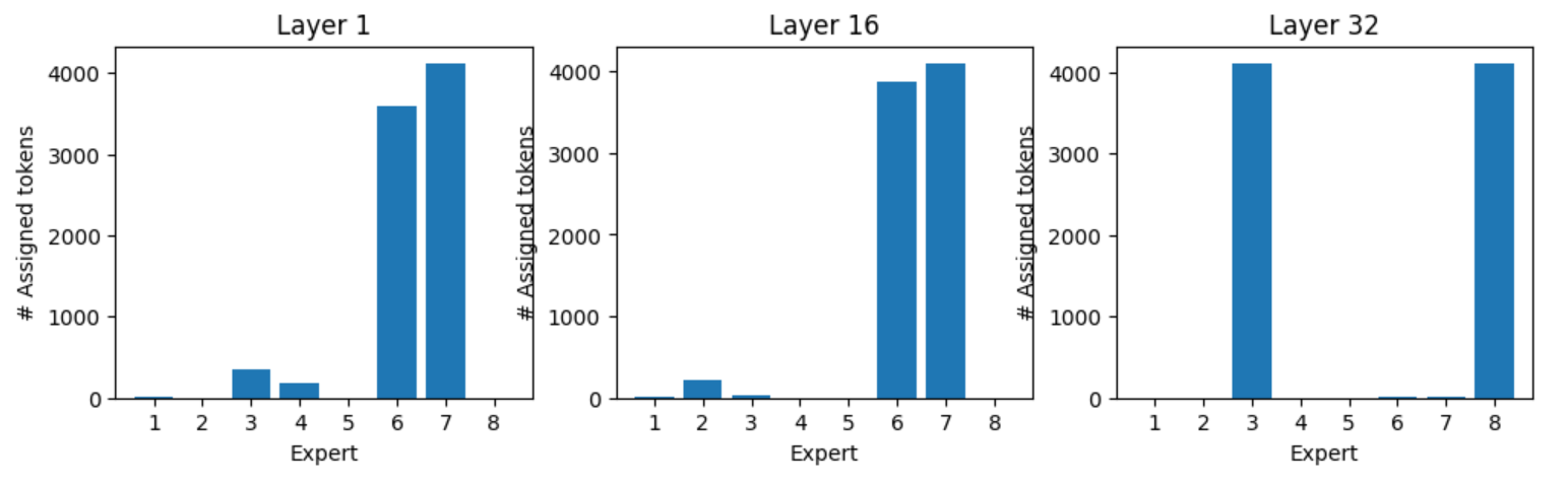
1
	**Figure 9. Expert assignment for token “.”**
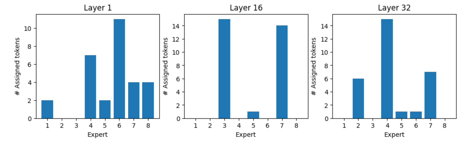
1
	**Figure 10. Expert assignment for token “what”**
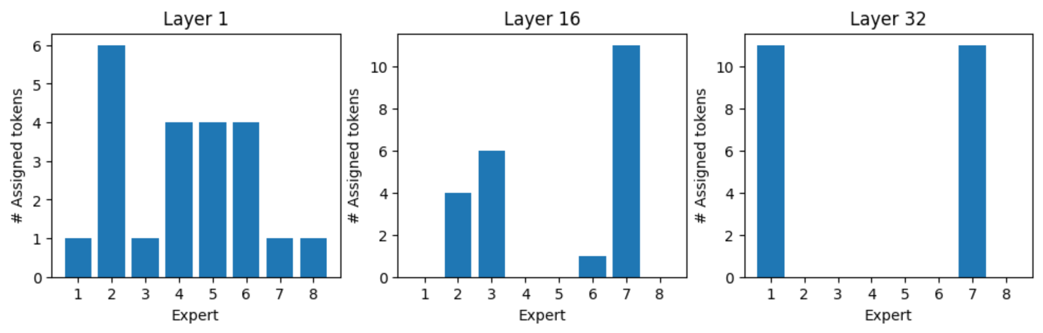
1
	**Figure 11. Expert assignment for token “who”**
Summary
MoE models provide demonstrable benefits to model pretraining throughput, enabling a more expressive sparse MoE model to be trained on the same amount of compute as a dense model. This leads to more competitive models under the same compute budget. MoE models can target the entire network, or specific layers within the existing network. Generally, sparse MoE with routing is applied to ensure that only some experts are used.
Our experiments explore how tokens are assigned and the relative load balance between experts. These experiments show that despite the load-balancing algorithm, there could still be large distributional imbalances, potentially affecting inference inefficiency, as some experts finish their work early while others are overloaded. This is an interesting area of active research.
You can try Mixtral 8x7B Instruct, as well as other AI models on build.nvidia.com.
Want to learn more? Don’t miss the panel session, Mistral AI: Frontier AI in Your Hands from NVIDIA GTC.
Learn how NVIDIA Blackwell NVL72 runs 10x faster and delivers 1/10 the token cost for MoE models in this blog.
第二部分:解析(深度解读)
核心论点
混合专家(Mixture of Experts, MoE)是一种神经网络架构模式:把某一层(线性层、MLP 或注意力投影)的计算拆成多个「专家」子网络,各自独立计算后再合并输出。它分两种:
- Dense MoE:每个输入都用到全部专家;
- Sparse MoE:每个输入只激活一部分专家。
MoE 的精髓在于「参数容量」与「每 token 计算量」的解耦——用更多的参数(专家)撑大模型容量,却只让其中一小部分参与每个 token 的前向计算,从而在相似模型规模下比稠密模型更省 FLOPs、更低延迟。Mixtral 8x7B 的开源,让社区首次得以在真实模型上实证专家的行为。
关键概念
- 模型容量(model capacity):MoE 层可替换普通层来扩大容量,而计算成本不随专家数线性增长。
- 注意力层共享,FFN 变 MoE:在典型 Transformer 中,注意力层通常所有 token 共享,前馈(FFN)层被替换为含 N 个专家 + 一个路由器(gating/router)的 MoE 层;路由器决定每个 token 交给哪几个专家。
- 负载均衡(load balancing):为防止少数专家被过度激活、其余「饿死」,训练时会加入负载均衡损失。但即便有该损失,专家仍会自发专业化。
- 专家专业化(expert specialization):在领域层面(domain)与 token 层面(token)同时显现。
实验发现(Mixtral 8x7B)
- 专家按领域/ token 专业化:尽管有负载均衡,特定专家仍更常被特定主题激活;实验显示 token 分布在「被均衡化」的同时仍有明显不均衡(如第 32 层的 expert 4 与 8 在抽象代数上接收了更多 token)。
- 特定 token 有偏好专家:标点与疑问词呈现强偏好——如
:、.、what、who各自对应稳定的专家分配(见正文柱状图)。 - 最常用 token / 最受偏好专家:词云与柱状图显示,不同专家「偏爱」的 token 集合高度分化。
技术趋势与判断
- MoE 已成前沿 LLM 主流:GPT-4、Mixtral、Qwen 等均以 MoE 为核心架构。其代价是训练/推理基础设施更复杂(路由、all-to-all 通信、专家并行),收益是推理成本大幅下降。
- 与硬件的耦合:MoE 每 token 激活参数少,对推理显存/带宽更友好;但专家间的 all-to-all 通信对芯片互联带宽提出新要求。NVIDIA 的 TensorRT-LLM、Dynamo、Blackwell NVL72 都围绕 MoE 做了专门优化(如宣称 MoE 推理 token 成本降至 1/10)。
- 呼应本模型效率主线:MoE 的「专家=事实存储」视角,与本站「模型正被刻意变笨(用知识换推理)」一文形成互补——专家层里大量参数正是被「外置/可选化」的知识存储。
与本站其他文章的连接
- 与「Models Are Getting Dumber on Purpose」互为注脚:稀疏激活让「小激活参数 + 大专家存储」成为可能,正是该文所述趋势的工程实现。
- 与「AI 硬件 / 推理芯片」主线相关:MoE 改变了推理的算力-带宽权衡,影响 H100 / Blackwell 及 CPO 光互联的需求结构。
风险提示
- 文章出自 NVIDIA 技术博客,带有推广其软件栈(TensorRT-LLM、Dynamo)的视角;结论应结合社区(如 Mistral、开源复现)独立验证。
- 负载均衡与路由机制仍是活跃研究方向,文中结论基于 Mixtral 8x7B 的具体实现,未必泛化到所有 MoE 变体。